Лако-красочные материалы — производство

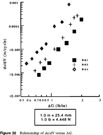
So far, only the load ratio effects on fatigue fracture of the FRP-wood interface have been investigated [7]. The log-log plot of the crack propagation rate da/dN versus the strain energy release rate range AG for load ratios R of 0.1, 0.3, and 0.5 is shown in Fig. 22. It is easily seen that there is a strong effect of load ratio R on crack propagation rate da/dN. The Crack propagation rate da/dN increases for the same strain energy release rate range, AG, when the load ratio increases. For each load ratio R, the following equation is used to fit the data points in Fig. 22:

where the constants B and m are obtained by regression fitting of experimental data and are listed in Table 11. As seen in Table 11, both B and m increase as the load ratio R increases. The relationship between crack propagation rate da/dN and minimum strain energy release rate Gmin is plotted in Fig. 23. Compared with Fig. 22, the load ratio effect on crack propagation rate da/dN in Fig. 23 is reversed; as the load ratio R increases, the crack propagation rate da/dN decreases for the same minimum strain energy release

rate Gmin.

As noticed by other researchers [20], the strain energy release rate range AG is not the only controlling parameter for the crack propagation rate da/dN. Since the minimum strain energy release rate Gmin and strain energy release rate range AG have contrary effects on the crack propagation rate da/dN for different load ratios R, the minimum strain energy release rate Gmin was included as a secondary controlling parameter to explain the load ratio effect. By following a similar approach as Hojo et al. [20], the equivalent strain energy release rate can be first defined as

A Geq = A G^G^n (7)

Then the modified Paris Law equation is expressed as

B( A Geq)m

In Eq. (7), 1 is a material constant that defines the relative importance of the contribution of the minimum strain energy release rate Gmin and strain energy release rate range AG to the crack growth rate. The constant 1 is obtained by a trial and error method to best fit the data points. The final log-log plot is shown in Fig. 24, for 1 = 0.13, B = 7 x 10“5, and m = 5.34 [7].